Investigating the field caused by a permanent magnet no free currents or time varying electric fields have to be considered. Thus, for the magnetic strength \(\vec{H}\) the following applies:
$$ \vec{\nabla} \times \vec{H} = 0. $$
Because of this, \(\vec{H}\) can be written as the gradient of a potential \(\Phi\):
$$ -\vec{\nabla} \Phi = \vec{H}. $$
Furthermore, the magnetic flux density has no sources:
$$ \vec{\nabla} \cdot \vec{B} = 0. $$
Magnetic flux density, magnetic field and magnetization are connected via:
$$ \vec{B} = \mu_0 (\vec{H} + \vec{M}). $$
Forming the divergence on both sides of the equals sign gives:
$$ div\vec{H} = -div\vec{M}. $$
In this formula, the mangetic field \(\vec{H}\) can be replaced by the gradient of the potential \( -\vec{\nabla} \Phi \):
$$ div(\vec{\nabla}\Phi) = div\vec{M}. $$
The equation has the form of Poisson's equation:
$$ \Delta \Phi = div \vec{M}. $$
Similar to the proceeding in the electrostatic case, this differential euqation can be solved by applying Green's theorem. The general solution is:
$$ \Phi(\vec{r}) = -\frac{1}{4\pi} \int \frac{div(\vec{M})}{|\vec{r}-\vec{r'}|} dV'. $$
Thereby, the integration is carried out over the volume of the magnet.
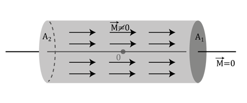
Figure 1 shows the magnet. The magnetization inside is constant \( \vec{M}=\begin{pmatrix} M_x \\ 0 \\ 0 \end{pmatrix} \) and outside constant \(0\). The change of the magnetization occurs on the end surfaces of the magnet. Therefore, the sources of the magnetization are on those surfaces. For further calculations, the expression for the divergence should be transformed into an expression for the surface divergence. The integration then just has to be carried out over the end faces of the magnet.
Furthermor, Figure 1 shows that on face \(A_1\) the magnetization changes from \(M_x\) to \(0\) and - vice versa - on face \(A_2\) from \(0\) to \(M_x\). For the surface divergence it follows:
$$ div_{surf}(\vec{M})|_{A_1} = -M_x \\ div_{surf}(\vec{M})|_{A_2} = M_x. $$
This results in (for more information, see Kemmer, 1977):
$$ \Phi(\vec{r}) = -\frac{1}{4\pi} \int_{A_1} \frac{-M_x}{|\vec{r}-\vec{r'}|} dA' -\frac{1}{4\pi} \int_{A_2} \frac{M_x}{|\vec{r}-\vec{r'}|} dA'. $$
The vector to the point at which the magnetic field is calculated is \( \vec{r} \). The vector to a point on the end faces of the magnet is \( \vec{r'} \). Because of the symmetry of the magnet, polar coordinates will be used for further proceedings.
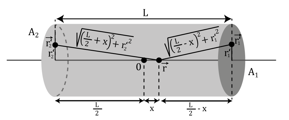
Figure 2 shows, how \( |\vec{r}-\vec{r'}| \) can be replaced by an integrable expression. It follows:
$$ \Phi(x) = \frac{1}{4\pi} \int_{0}^{2\pi}d\phi \int_{0}^{R}dr'_1 r'_1 \frac{M_x}{\sqrt{(\frac{1}{2}L - x)^2+{r'_1}^2}} - \frac{1}{4\pi} \int_{0}^{2\pi}d\phi \int_{0}^{R}dr'_2 r'_2 \frac{M_x}{\sqrt{(\frac{1}{2}L + x)^2+{r'}_2^2} }. $$
By using \( \int_{a}^{b} dr \frac{r}{\sqrt{c + r^2}} = \sqrt{c+r^2}|^b_a \) the integral can be calculated:
$$ \Phi(x) = \frac{1}{2}M_x \left( \left[\sqrt{(\frac{1}{2}L - x)^2+{r'_1}^2} \right] _0^R \right) - \frac{1}{2}M_x \left( \left[\sqrt{(\frac{1}{2}L + x)^2+{r'_2}^2} \right] _0^R \right) $$
$$ = \frac{1}{2}M_x \left( \sqrt{(\frac{1}{2}L - x)^2 + R^2} - \sqrt{(\frac{1}{2}L-x)^2} - \sqrt{(\frac{1}{2}L+x)^2 + R^2} + \sqrt{(\frac{1}{2}L+x)^2} \right). $$
$$ = \frac{1}{2}M_x \left( \sqrt{(\frac{1}{2}L - x)^2 + R^2} - \left|\frac{1}{2}L-x\right| - \sqrt{(\frac{1}{2}L+x)^2 + R^2} + \left|\frac{1}{2}L+x\right| \right). $$
Using \( \Phi(x) \), \( \vec{H} \) along the x-axis can be calculated:
$$ \vec{H}(x) = -\vec{\nabla}\Phi(x) = -\frac{\partial}{\partial x} \Phi(x) \vec{e}_x \\ $$
$$ =-\frac{1}{2}M_x \left( - \frac{\frac{1}{2}L-x}{\sqrt{(\frac{1}{2}L-x)^2 + R^2}} + \frac{\frac{1}{2}L-x}{\sqrt{(\frac{1}{2}L-x)^2}} - \frac{\frac{1}{2}L+x}{\sqrt{(\frac{1}{2}L+x)^2 + R^2}} + \frac{\frac{1}{2}L+x}{\sqrt{(\frac{1}{2} L+x)^2}} \right) \vec{e}_x $$
$$ =-\frac{1}{2}M_x \left( - \frac{\frac{1}{2}L-x}{\sqrt{(\frac{1}{2}L-x)^2 + R^2}} + \frac{\frac{1}{2}L-x}{\left|\frac{1}{2}L-x\right|} - \frac{\frac{1}{2}L+x}{\sqrt{(\frac{1}{2}L+x)^2 + R^2}} + \frac{\frac{1}{2}L+x}{\left|\frac{1}{2} L+x\right|} \right) \vec{e}_x. $$
For points \( \vec{r} \) outside the magnet \( |x|>\frac{L}{2} \). This yields:
$$ \vec{H}(x) =\frac{1}{2}M_x \left( \frac{\frac{1}{2}L-x}{\sqrt{(\frac{1}{2}L-x)^2 + R^2}} + \frac{\frac{1}{2}L+x}{\sqrt{(\frac{1}{2}L+x)^2 + R^2}} \right)\vec{e}_x. $$
For points inside the magnet \( |x| \lt \frac{L}{2} \), which gives:
$$ \vec{H}(x) =\frac{1}{2}M_x \left( \frac{\frac{1}{2}L-x}{\sqrt{(\frac{1}{2}L-x)^2 + R^2}} + \frac{\frac{1}{2}L+x}{\sqrt{(\frac{1}{2}L+x)^2 + R^2}} -2 \right)\vec{e}_x. $$
For the mangetic flux density outside the magnet \( \vec{B}=\mu_0 \vec{H} \) holds and so:
$$ \vec{B}(x) =\frac{1}{2}M_x\mu_0 \left( \frac{\frac{1}{2}L-x}{\sqrt{(\frac{1}{2}L-x)^2 + R^2}} + \frac{\frac{1}{2}L+x}{\sqrt{(\frac{1}{2}L+x)^2 + R^2}}\right)\vec{e}_x. $$
Using \(\vec{B} = \mu_0 (\vec{H} + \vec{M}) \) and the formula for \(\vec{H}(x)\) it can be seen that this dependence even describes the magnetic flux density inside the manget (see also Sommerfeld, 1956).
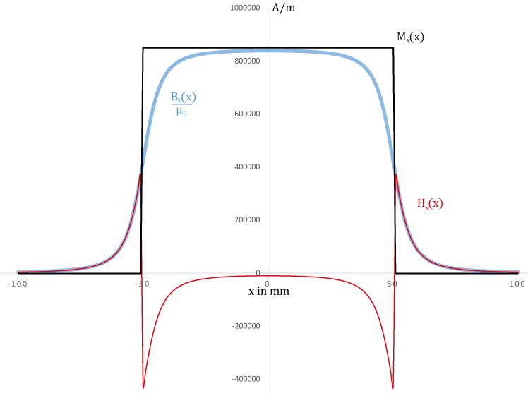
The used magnet is of length \( L=100mm \) und radius \( R=7.5mm \). Figure 3 shows the graphs of the magnetization, the magnetic field and the magnetic flux density for a magnetization of \( M_x(x)|_{-\frac{L}{2} \leqslant x \leqslant \frac{L}{2}} = 850\frac{\mathrm{kA}}{\mathrm{m}} \). For the presentation in the diagram the magnetic flux density was divided by the magnetic field constant \(\mu_0\).